


So many other frameworks exist, why MXNet?
is a modern interpretation and rewrite of a number of ideas being talked about in the deep learning infrastructure. It’s designed from the ground up to work well with multiple GPUs and multiple computers.
When doing multi-device work in other frameworks, the end user frequently has to think about when to do computation and how data is synchronized. In MXNet, every operation is lazy. It only computes values when the resources are available to compute them.
In practice, you get incredible device utilization automatically. A new batch can be copying to a GPU, while that same GPU can be running a forward pass as a CPU does a complex parameter update on the CPU — all at the same time!
In addition:
- It is built on a dataflow graph (like Tensorflow, Theano, Torch, Caffe).
- It manages its own memory internally (like Theano) and is able to reuse memory locations.
- It has a backend written in C++ and cuda, which is exported via a C interface. This allows simple language bindings. It currently supports Python, R, Julia, Go and Javascript (in varying degrees).
- It allows use of Torch natively from Python.
- It can be deployed on mobile.
For a high level overview of MXNet, check out their Arxiv Paper.
Imperative vs. Symbolic
There are two modes of computation in MXNet: imperative and symbolic. The imperative API exposes an interface similarly to Numpy. The symbolic API lets users define computation graphs, similar to Theano and Tensorflow.
Imperative
The basic building block for the imperative API is an NDArray. Much like Numpy, this object holds a tensor (or multi-dimensional array). Unlike Numpy, this object also stores a pointer to where the memory is held (CPU or GPU).
For example, to construct a tensor of zeros on CPU and GPU:
import mxnet as mx
cpu_tensor = mx.nd.zeros((10,), ctx=mx.cpu())
gpu_tensor = mx.nd.zeros((10,), ctx=mx.gpu(0))
In MXNet, you need to specify where arrays are held. This is done by passing in an appropriate context to GPU or CPU.
Much like in Numpy, basic math operations can be done on these.
ctx = mx.cpu() # which context to put memory on.
a = mx.nd.ones((10, ), ctx=ctx)
b = mx.nd.ones((10, ), ctx=ctx)
c = (a + b) / 10.
d = b + 1

d, you need to know the value of b, so that must be computed first. In this example, you don’t need to know the value of c to compute d, meaning that the execution engine is free to compute c and d in whatever order it wants, or even concurrently in an efficient manner.
To actually read the values in the NDArray, you can call:
numpy_d = d.asnumpy()
This function blocks until the value of d has been computed, then converts it to a Numpy array.
Symbolic
While the imperative API is extremely powerful by itself, it is often very rigid and hard to prototype with. Everything must be known about the computation ahead of time, and must be written out by the user. The symbolic API tries to remedy this. Instead of working with defined arrays, you work with symbols that can be “compiled” or interpreted to a executable set of operations.
Take a similar example to the one above:
import mxnet as mx
a = mx.sym.Variable("A") # represent a placeholder. These can be inputs, weights, or anything else.
b = mx.sym.Variable("B")
c = (a + b) / 10
d = c + 1
With these symbols defined, we can inspect the graph’s inputs and outputs.
d.list_arguments()
# ['A', 'B']
d.list_outputs()
# ['_plusscalar0_output'] This is the default name from adding to scalar.
The graph allows shape inference.
# define input shapes
inp_shapes = {'A':(10,), 'B':(10,)}
arg_shapes, out_shapes, aux_shapes = d.infer_shape(**inp_shapes)
arg_shapes # the shapes of all the inputs to the graph. Order matches d.list_arguments()
# [(10, ), (10, )]
out_shapes # the shapes of all outputs. Order matches d.list_outputs()
# [(10, )]
aux_shapes # the shapes of auxiliary variables. These are variables that are not trainable such as batch normalization population statistics. For now, they are save to ignore.
# []
Stateless Graphs
Unlike other frameworks, MXNet’s graphs are completely stateless. They just represent some function that has arguments and outputs. In MXNet there is no difference between “weights”, or parameters of a model and its inputs (data fed in). They are both arguments to the graph. For example, a graph representing a logistic regression would have three arguments: the input data, some weights, and biases.
To actually perform computation in the graph, we need to create what MXNet calls an Executor. This can be done by bind-ing an output symbol with a specific set of input variables.
input_arguments = {}
input_arguments['A'] = mx.nd.ones((10, ), ctx=mx.cpu())
input_arguments['B'] = mx.nd.ones((10, ), ctx=mx.cpu())
executor = d.bind(ctx=mx.cpu(),
                  args=input_arguments, # this can be a list or a dictionary mapping names of inputs to NDArray
                  grad_req='null') # don't request gradients
This Executor allocates all the necessary memory and temporary variables to perform the computation. Once bound, an Executor always works with the same memory locations for inputs and outputs. To actually compute results for given values, you need to modify the contents of the input variables, call forward, and then read out the outputs.
import numpy as np
# The executor
executor.arg_dict
# {'A': NDArray, 'B': NDArray}
executor.arg_dict['A'][:] = np.random.rand(10,) # Note the [:]. This sets the contents of the array instead of setting the array to a new value instead of overwriting the variable.
executor.arg_dict['B'][:] = np.random.rand(10,)
executor.forward()
executor.outputs
# [NDArray]
output_value = executor.outputs[0].asnumpy()
Like in the imperative API, calling forward is also lazy and will return before computation is finished.
Now, the great thing about doing computation with a dataflow graph is that you can automatically differentiate with respect to inputs. This can be done automatically with the backward function. The Executor needs a place to put the output gradients though for this to work, as shown below.
# allocate space for inputs
input_arguments = {}
input_arguments['A'] = mx.nd.ones((10, ), ctx=mx.cpu())
input_arguments['B'] = mx.nd.ones((10, ), ctx=mx.cpu())
# allocate space for gradients
grad_arguments = {}
grad_arguments['A'] = mx.nd.ones((10, ), ctx=mx.cpu())
grad_arguments['B'] = mx.nd.ones((10, ), ctx=mx.cpu())
executor = d.bind(ctx=mx.cpu(),
                  args=input_arguments, # this can be a list or a dictionary mapping names of inputs to NDArray
                  args_grad=grad_arguments, # this can be a list or a dictionary mapping names of inputs to NDArray
                  grad_req='write') # instead of null, tell the executor to write gradients. This replaces the contents of grad_arguments with the gradients computed.
executor.arg_dict['A'][:] = np.random.rand(10,)
executor.arg_dict['B'][:] = np.random.rand(10,)
executor.forward()
# in this particular example, the output symbol is not a scalar or loss symbol.
# Thus taking its gradient is not possible.
# What is commonly done instead is to feed in the gradient from a future computation.
# this is essentially how backpropagation works.
out_grad = mx.nd.ones((10,), ctx=mx.cpu())
executor.backward([out_grad]) # because the graph only has one output, only one output grad is needed.
executor.grad_arrays
# [NDarray, NDArray]
Flexibility vs. Complex interfaces
One of MXNet’s design goals is to be flexible. As a result, it often exposes APIs at multiple different levels. The above call to bind needs all input and gradient arguments defined before hand. A lot of this information could be calculated using shape inference. A simpler API, simple_bind, also exists for the same task. This allocates all the necessary space needed. All it needs is a few input shapes to fully specify the graph.
input_shapes = {'A': (10,), 'B': (10, )}
executor = d.simple_bind(ctx=mx.cpu(),
                         grad_req='write', # instead of null, tell the executor to write gradients
                         **input_shapes)
executor.arg_dict['A'][:] = np.random.rand(10,)
executor.arg_dict['B'][:] = np.random.rand(10,)
executor.forward()
out_grad = mx.nd.ones((10,), ctx=mx.cpu())
executor.backward([out_grad])
Power of Combining Imperative and Symbolic
The real power of MXNet is that you can combine the two styles.
For example, you can use symbolic operations to construct a neural network. Bind an executor to compute for a given batch_size, then use the imperative API to do gradient updates. All of these operations will be performed lazily when the needed data is available.
Now for a more complicated example: a small, fully connected neural network with one hidden layer for MNIST.
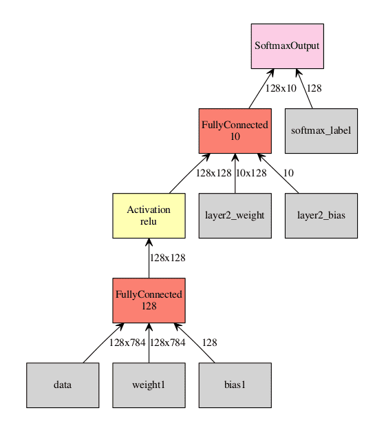
Visualization of the network. Inputs to the graph are in gray, all other squares are operations performed on the inputs. In this example we are using a batch size of 128.
import mxnet as mx
import numpy as np
# First, the symbol needs to be defined
data = mx.sym.Variable("data") # input features, mxnet commonly calls this 'data'
label = mx.sym.Variable("softmax_label")
# One can either manually specify all the inputs to ops (data, weight and bias)
w1 = mx.sym.Variable("weight1")
b1 = mx.sym.Variable("bias1")
l1 = mx.sym.FullyConnected(data=data, num_hidden=128, name="layer1", weight=w1, bias=b1)
a1 = mx.sym.Activation(data=l1, act_type="relu", name="act1")
# Or let MXNet automatically create the needed arguments to ops
l2 = mx.sym.FullyConnected(data=a1, num_hidden=10, name="layer2")
# Create some loss symbol
cost_classification = mx.sym.SoftmaxOutput(data=l2, label=label)
# Bind an executor of a given batch size to do forward pass and get gradients
batch_size = 128
input_shapes = {"data": (batch_size, 28*28), "softmax_label": (batch_size, )}
executor = cost_classification.simple_bind(ctx=mx.gpu(0),
                                           grad_req='write',
                                           **input_shapes)
# The above executor computes gradients. When evaluating test data we don't need this.
# We want this executor to share weights with the above one, so we will use bind
# (instead of simple_bind) and use the other executor's arguments.
executor_test = cost_classification.bind(ctx=mx.gpu(0),
                                         grad_req='null',
                                         args=executor.arg_arrays)
# initialize the weights
for r in executor.arg_arrays:
    r[:] = np.random.randn(*r.shape)*0.02
# Using skdata to get mnist data. This is for portability. Can sub in any data loading you like.
from skdata.mnist.views import OfficialVectorClassification
data = OfficialVectorClassification()
trIdx = data.sel_idxs[:]
teIdx = data.val_idxs[:]
for epoch in range(10):
  print "Starting epoch", epoch
  np.random.shuffle(trIdx)
  for x in range(0, len(trIdx), batch_size):
    # extract a batch from mnist
    batchX = data.all_vectors[trIdx[x:x+batch_size]]
    batchY = data.all_labels[trIdx[x:x+batch_size]]
    # our executor was bound to 128 size. Throw out non matching batches.
    if batchX.shape[0] != batch_size:
        continue
    # Store batch in executor 'data'
    executor.arg_dict['data'][:] = batchX / 255.
    # Store label's in 'softmax_label'
    executor.arg_dict['softmax_label'][:] = batchY
    executor.forward()
    executor.backward()
    # do weight updates in imperative
    for pname, W, G in zip(cost_classification.list_arguments(), executor.arg_arrays, executor.grad_arrays):
        # Don't update inputs
        # MXNet makes no distinction between weights and data.
        if pname in ['data', 'softmax_label']:
            continue
        # what ever fancy update to modify the parameters
        W[:] = W - G * .001
  # Evaluation at each epoch
  num_correct = 0
  num_total = 0
  for x in range(0, len(teIdx), batch_size):
    batchX = data.all_vectors[teIdx[x:x+batch_size]]
    batchY = data.all_labels[teIdx[x:x+batch_size]]
    if batchX.shape[0] != batch_size:
        continue
    # use the test executor as we don't care about gradients
    executor_test.arg_dict['data'][:] = batchX / 255.
    executor_test.forward()
    num_correct += sum(batchY == np.argmax(executor_test.outputs[0].asnumpy(), axis=1))
    num_total += len(batchY)
  print "Accuracy thus far", num_correct / float(num_total)
MXNet does contain a whole host of higher level APIs to dramatically reduce complexity of more straight forward models like the one above. Here is an example of the same model using the FeedForward class. A lot more is hidden, but the code is a lot smaller and simpler.
import mxnet as mx
import numpy as np
import logging
logging.basicConfig(level=logging.INFO)
logger = logging.getLogger(__name__) # get a logger to accuracies are printed
data = mx.sym.Variable("data") # input features, when using FeedForward this must be called data
label = mx.sym.Variable("softmax_label") # use this name aswell when using FeedForward
# When using Forward its best to have mxnet create its own variables.
# The names of them are used for initializations.
l1 = mx.sym.FullyConnected(data=data, num_hidden=128, name="layer1")
a1 = mx.sym.Activation(data=l1, act_type="relu", name="act1")
l2 = mx.sym.FullyConnected(data=a1, num_hidden=10, name="layer2")
cost_classification = mx.sym.SoftmaxOutput(data=l2, label=label)
from skdata.mnist.views import OfficialVectorClassification
data = OfficialVectorClassification()
trIdx = data.sel_idxs[:]
teIdx = data.val_idxs[:]
model = mx.model.FeedForward(symbol=cost_classification,
                             num_epoch=10,
                             ctx=mx.gpu(0),
                             learning_rate=0.001)
model.fit(X=data.all_vectors[trIdx],
          y=data.all_labels[trIdx],
          eval_data=(data.all_vectors[teIdx], data.all_labels[teIdx]),
          eval_metric="acc",
          logger=logger)
Conclusion
I hope this tutorial has been a good introduction to MXNet at its core. Personally, I find this low level of work essential when trying out the latest research work. In general, with almost all of these frameworks, there is a trade off between how expressive you must be (how much code you have to write), and flexibility to implement new and unthought of techniques.
I’ve only scratched the surface of what is inside MXNet — for more information check out the docs. They include both documentation on how to use MXNet as well as design notes from the developers. If you have any questions, feel free to reach out to contact@indico.io! We’re always happy to chat.