In the frothy sea of Big Data buzz, there’s a tidbit: “More data beats a better model.” But if you’re not Google, and you’re not building distributed language models…well, haven’t you ever wondered how much improvement a model should yield when scaling up to a bigger dataset? Here we look at a specific example to see how it really depends on the task, your data, and your models — and how the promised improvements probably aren’t as dramatic as you think.Most organizations:
- Have less data than you might assume.
- Of the data you have, only a fraction is relevant for solving a problem that matters.
- Of the relevant data, only a fraction is usable and structured to feed a model.
- Of the relevant and usable data, only a fraction of the observations are encoding useful information that be exploited by a model.
So…why all the focus on bytes?
Because it’s easy, not because it’s useful.
Since storage became cheap, industry practice is to collect everything and sort it out later. The problem is, you never do. Time marches on, and you find yourself just as busy today as you were before…plus now you have a big, messy dataset that requires even more time and effort to handle. Nobody in the organization can quantify the utility of your data assets, so when someone is forced to give metrics to show how the organization is doing Big Data™, it is really easy to report metrics on data storage—so many bytes! And sure, that’s an easy metric to compute, but it’s also a really weak measure.
Data storage metrics are weak because they tell you very little about the value or utility of the observations being stored with those bytes. For example, storing duplicate observations takes twice the storage space, for zero benefit. Rather than size-on-disk, a much better metric to quantify your data assets is coverage:
You should define coverage in terms of the problem or use case your organization is solving, and it is OK to estimate things. Since we’re talking about “big data”, let’s use a fair example: unstructured text. We’ll work through a specific example, using a well-defined task (sentiment analysis) and a massively diverse dataset (online reviews written in English) to see what happens when we train models with increasingly large amounts of input data. But first, check your own intuition! How much data will be required to double the accuracy of a sentiment model? Doubling the data? 3X? 10X? 100X? (Guess now, then keep reading!)
Case study:
A specific example to illustrate the trade-offs between data and model complexity.
The task:
Our task will be sentiment analysis—given a chunk of text, classify the text as expressing either positive or negative feelings.
Note: The next few sections get a bit technical, so feel free to skip to the Results section at any point to see how the model changes as more data is added.
Data:
We’ll use online reviews, which have been labeled (by human reviewers) as positive or negative. Specifically, these reviews were written in English, and include typos and all the other messiness inherent to online data. To show the effects of scaling input data, the dataset was divided into chunks. This allows us to train models on increasingly larger sets of input data (i.e., the next training dataset is the previous dataset, plus a chunk of fresh data). Data were further split into training and test sets. To ensure the test metrics are a fair representation of model performance, each test set was held out from the training process, and used only to evaluate performance of the models.
The model:
We’ll use a model that is both straightforward to train and surprisingly effective: logistic regression on TF-IDF (term frequency – inverse document frequency) bi-gram features (i.e., pairs of words). Basically, a model counts how often words occur in the training data, in order to learn which words are associated with positive or negative labels. To train the model, we scan across the training data, counting pairs of words. Then we feed these vectors (of word frequencies) into a logistic regression model, to learn how pairs of words are associated with positive versus negative labels.
Once the model is trained, to evaluate the sentiment of text, we vectorize the text into word counts in the same way, and use the trained model to compute a probability that the text is positive (or negative). To ensure we’re working with good values for each parameter, we performed a grid search over model hyperparameters. Regularization parameters were purposefully chosen to overfit the data, allowing us to isolate the effects of input data, as we scale from 1X to 100X.
Evaluation:
To evaluate predictive power, we want to score correct vs. false predictions, so we’ll use accuracy and the Receiver Operating Characteristic (ROC). Accuracy is simply the fraction of correct predictions, which are evaluated on the test data. ROC shows the true positive rate as a function of the false positive rate, so it helps us understand how the model is balancing sensitivity (i.e., can it find all the true predictions?) versus specificity (i.e., can it avoid making false predictions?).
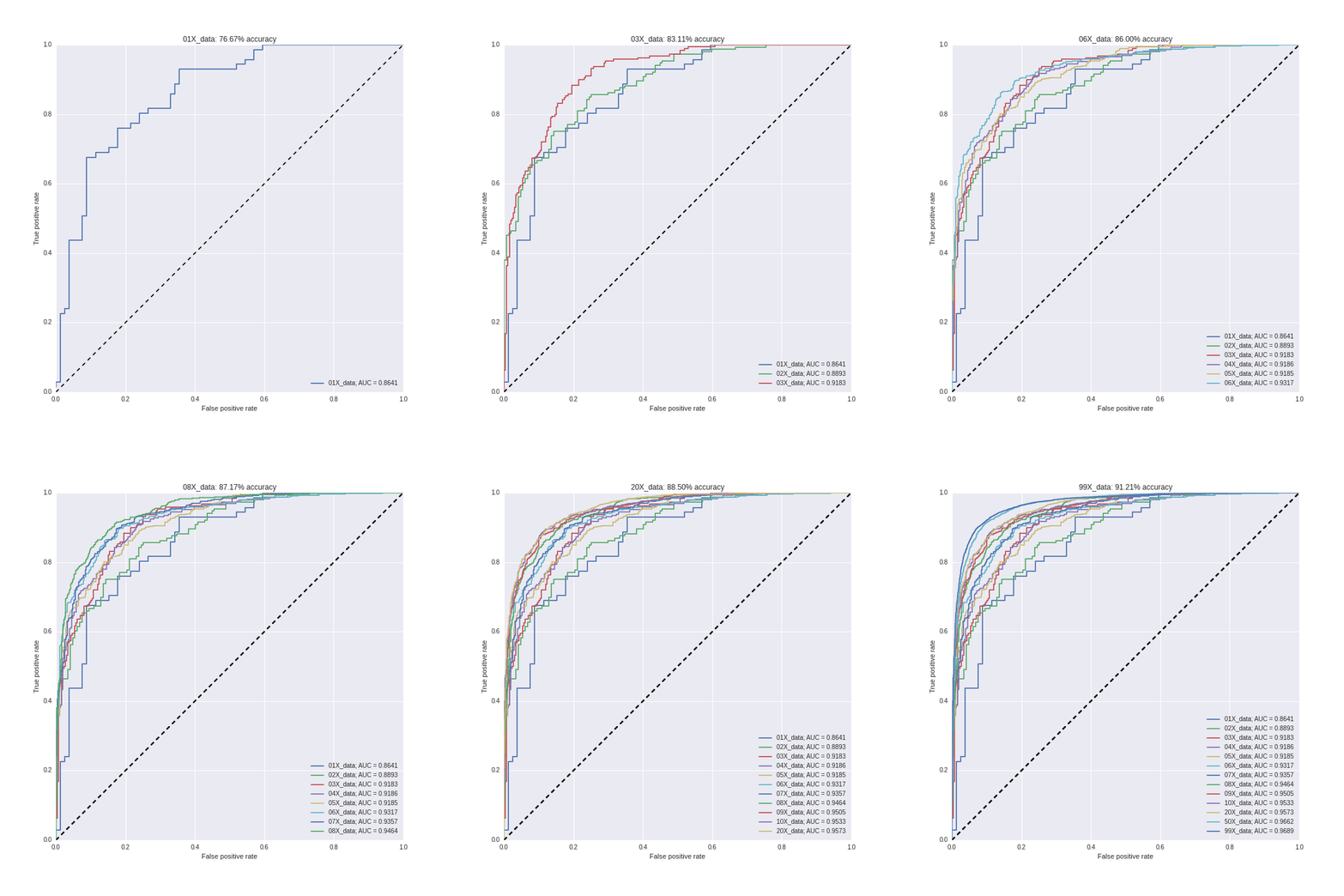
A random model would have an equal chance to make a correct vs. false prediction, tracing out the diagonal dashed line on the ROC plot (see Figure 1 below). A perfect model would immediately choose the correct predictions, with a curve following the top left of the ROC plot. Real models are somewhere between random and perfect, and we expect to see the curve moving up and to the left as models become more powerful.
Figure 1. This Receiver Operating Characteristic (ROC) curve illustrates how the predictive power of a straightforward text sentiment prediction model scales with the amount of training data. A model making random predictions would follow the dashed diagonal; better predictions go farther up and left. 1X data is approximately 8 million words, from randomly sampled online reviews. The animation was made so that the time to add a new line to the plot is proportional to the amount of new data added.
Results:
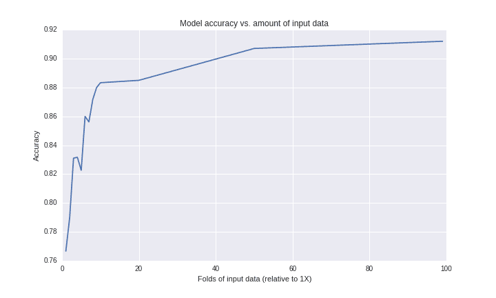
Figure 1 shows how increasing amounts of input data improve the predictive power of each model. In Figure 2, we see how adding more training data causes an initial burst of improvement to model accuracy, but then increasingly large amounts of data are required for even incremental gains. This is because there are many many ways to compose reviews using English, so we need to scan huge amounts of new data to find even a few new observations (i.e., new word pairs) to add to the model.
Finally, Figure 3 shows how the predictive power of the model scales as a function of input data. This is a relatively simple model, and we are illustrating a relatively small fraction of data compared to the full diversity of ways a review could be composed of words in English. Whereas it is clear that models improve as more data are used to train the model, it is clearly a case of diminishing returns, and this kind of model quickly becomes prohibitive.
So yes, the more data the better…until the exponential scaling forces you to accept the trade-offs, and that happens sooner than you might think. For some problems, it is worth throwing a ton of resources at the problem to get tiny improvements in predictive power, because that last percentage point is worth it! But you should engage in such an endeavor fully aware of the resources required to achieve those diminishing returns.
Figure 2. Accuracy as a function of the number of observations used to train the model. This graph shows how increasingly large quantities of input data are needed to add new words to the vocabulary. Note the logarithmic shape! Because bigger samples of data (i.e., English text) include a lot of redundant information, it becomes prohibitive to add useful information to the model. This particular example will likely approach (but never exceed) 92% accuracy. Some minor jaggedness is due to noise in the model, which could be alleviated using a different random seed, or smoothed across many folds of cross-validation.
Figure 3. This plot shows how predictive power (i.e., area under each of the ROC curves shown above in Figure 1) varies with the amount of input data; higher AUC values generally indicate stronger models. 1X data is approximately 8M English words (so, 100X data is approximately 800M words). Although training models with more data does yield stronger models, the improvements are asymptotic. This graph is useful for calibrating intuition—even if you have never trained a machine learning model, try visually extrapolating the trends here, to see how a much larger dataset will yield only a marginally better result!
More data are better, up to a point — and that point is less than you might think.
We hope you enjoyed this brief exploration of the tradeoffs machine learning teams encounter when building solutions. The power of “big data” isn’t about how many bytes you’re storing in your datacenter, but about how many useful observations you can apply to solve a specific problem. When you’re trying to build better features into a model, more data are indeed better, up to a point where adding new observations becomes prohibitive.
To improve beyond this point, you need better strategies to compute features, and better models to exploit them. For example, we could use a different model, such as one that composes features more effectively than n-grams. If you want to define your business needs as solvable machine learning projects, but find yourself (or your organization) stalling out, get in touch! We do this all the time and love hearing about use cases; we’d be happy to help you understand the factors and recommend solutions.


