

In part one, we showed how the machine learning process is like the scientific thinking process, and in part two, we introduced a benchmark task and showed how to get your machine learning system up and running with a simple nearest neighbors model.
Now you have all the necessary parts of a machine learning system:
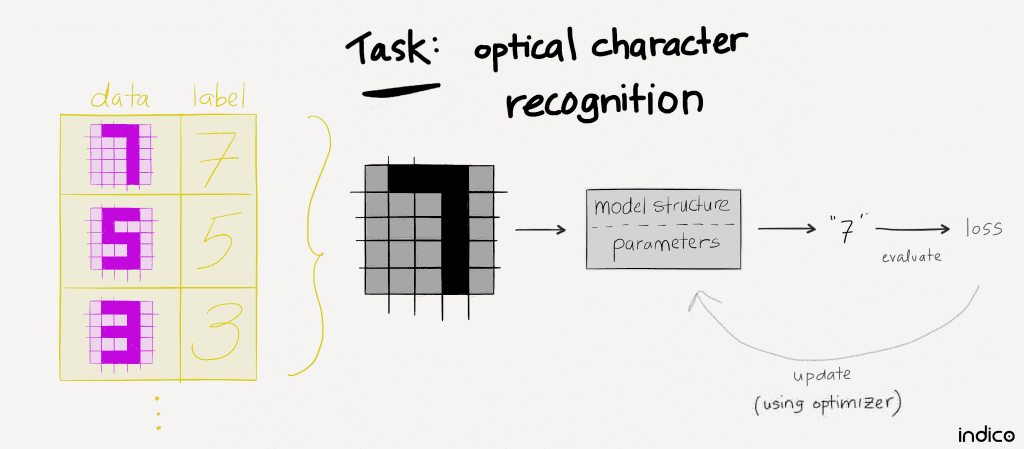
- A problem worth solving, defined as a specific machine learning task. Here we’re solving the task of optical character recognition, a 10-way classification task. Specifically, given a 28×28 grayscale image of a handwritten number, label it as the correct digit (e.g., “4”).
- Data + labels to feed our model.
- Model to represent and exploit knowledge for this data distribution and task. So far, we’ve only used the “nearest neighbors” model, which looks for the most similar example in the known dataset, and assumes the input has the same label as the known example.
- A principled way to evaluate and compare performance (i.e., evaluation metrics).
But maybe you are wondering…what about better models?
Time to crank it up! In this post, we continue the scientific thinking process by extending our simple starting model into increasingly powerful models.
via GIPHY
- Evaluate on a dataset that wasn’t used to train the model.
- Inspect the errors.
- Identify patterns of errors.
- Diagnose the patterns of errors, in the context of the model. What about the model led it to make the wrong predictions?
- Make a new hypothesis.
- Implement the new hypothesis as a new model.
- Train the new model.
- Visualize the result.
(…and iterate!)
Shortcutting this process is a common failure mode—ye’ve been warned! Experts practice exactly the same process, perhaps even more systematically. But familiarity with common patterns of errors, diagnoses, and solutions allow experts to zip through the iterations. From the perspective of someone who is learning, it might look like the expert is skipping steps and going straight to the complicated stuff. But that isn’t the case! Experts spend the most time working on complicated stuff because the simple stuff has been tried/solved already :).
There is no reason to assume your particular problem cannot be solved by simpler models until you have tested them. Simpler models have many benefits, so start simple! Skip around if you must, but make sure you understand how to practice the entire end-to-end scientific thinking process.
1. Evaluate predictions
To improve our machine learning system, we need to understand how the current system makes errors. Then we test a hypothesis (i.e., a new model) to see if we can eliminate errors.
When does the nearest neighbors model make mistakes? Let’s evaluate the first 1000 dev images, and inspect the examples where the nearest neighbor prediction was wrong.
dev_images = dev_images[0:1000]
dev_labels = dev_labels[0:1000]
pred = np.zeros(len(dev_images))
for i, query_image in tqdm(enumerate(dev_images)):
    pred[i] = nearest_neighbor(query_image)
acc = np.zeros(len(dev_images))
for i, pred_label in enumerate(pred):
    if int(pred_label) == int(dev_labels[i]):
        acc[i] = 1
    else:
        print("example %d: predicted %d, real answer is %d" % (i, pred[i], dev_labels[i]))
accuracy = acc.sum() / len(acc)
print("Accuracy: %.3f%%, evaluated on %d examples" % (accuracy * 100., len(acc)))
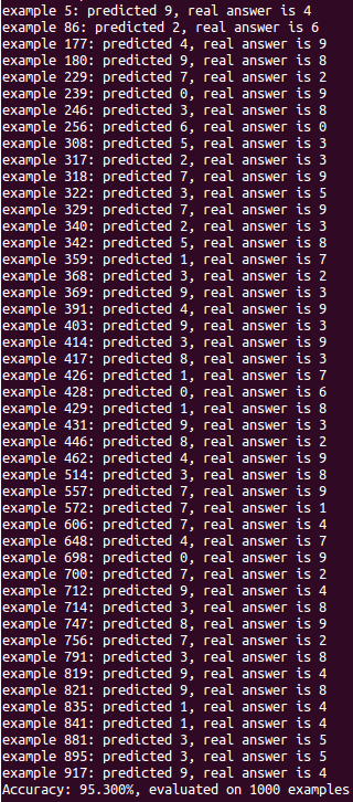
Evaluate the first 1000 dev examples.
47 mistakes ≈ 95.3% accuracy.
From just the predicted vs. real labels, can we start to understand why this model made mistakes? There do seem to be some patterns. For example, a handwritten 4 vs. 9 might have very similar pixels, depending on the roundness of the top loop. And perhaps there is a pattern to the predictions…it seems like 7, 9, and 1 are incorrectly predicted more frequently than others.
2. Inspect the errors
It is good to exercise intuition, but we can’t stop there! Now that we know which examples were incorrectly predicted, we can inspect the actual image data of those examples (feel free to inspect correct predictions too). Here are a few errors and a code snippet to do it for yourself:
from matplotlib import pyplot as plt
ex = 5  # change this value to whichever example you want to view
plt.imshow(dev_images[ex].reshape((28,28)), cmap = "gray_r")
plt.show()

Example 5: predicted 9, real answer is 4.
Maybe the model made a mistake because the overall shapes are similar,
but the sharp difference in a few pixels at the top of the loop are not enough
to overcome the rest of the shape (which looks very similar for 4 and 9).
Example 86: predicted 2, real answer is 6. Is this *my* handwriting? 😉
Just kidding. I don’t know what to make of this blob. Next!
Example 177: predicted 4, real answer is 9.
As in example 5 above, a sharp visual difference that spans only a few pixels
is not enough to overcome the overall similarity of the rest of the shape.
Example 180: predicted 9, real answer is 8.
Most of the pixels (the top loop) do look like a 9, but the bottom loop distinguishes it as an 8.
The bottom loop is relatively small here, but a nearest neighbors model doesn’t care.
3. Look for patterns of errors
OK, we’ve only shown a few illustrative images here, but we looked at many more, and encourage you to do the same. Observe the errors. Do you notice anything in common to these incorrectly predicted examples?
What patterns did you notice? We noticed how, in some examples, a small region of pixels can be very important for determining the correct digit. Where the discriminative part of the handwriting is small, and the overall stroke is ambiguous, the model makes mistakes.
4. Diagnose errors: how did the model make mistakes?
When a dataset is large and diverse, there are bound to be bad examples (e.g., example #86 in the figure above). But if we can detect a systematic pattern and understand how it happens in the specific context of this model and data distribution, then we can think about formulating a better hypothesis.
Many of the pixel locations, especially the border pixels, always have a value of 0. Other locations are more interesting.
So, now that we have identified a pattern of errors, how do we explain the pattern in the context of the model? It is great practice to think through this, please take a moment to express your thoughts before continuing on.
It can be helpful to write ideas on paper or whiteboard. Do whatever is most natural for you…draw something, sketch logical diagrams, or write words. For example:
We noticed errors where the overall stroke of handwriting might be similar to
an incorrect digit (green), and a small discriminative region (red)
is not able to overcome it.
Our explanation for the pattern of mistakes? In the nearest neighbors model, specifically in the sse_distance function, each pixel contributes equally to the prediction. But the useful information is not uniformly distributed across pixels. Some pixels are more informative than others, like the region at the top of the 9 vs. 4 in the figure above. Intuitively, this makes sense. When we humans read handwriting, we focus on specific parts of the stroke to discriminate one character from another. So yes, the errors make sense in the context of a nearest neighbors model! The model is being fooled when the discriminative regions of handwriting are small and the overall stroke shape is ambiguous.
Diagnosis: each pixel is a feature that could be exploited to make predictions, but the nearest neighbors model doesn’t have the ability to weight the informative pixels more strongly than other pixels.
5. Strategy to fix the errors -> a new hypothesis
Now that we have a hypothetical explanation for pattern of errors we have observed…can we think of a strategy to eliminate those errors? How would you change the model to give more predictive power to the discriminative regions of handwriting (regardless of size), while still being sensitive to the overall shape?
There are many possible strategies, and we encourage you to try a few :). One particularly useful strategy exploits the concept of weights. We give each pixel a weight parameter, so that the contribution of each pixel (to the prediction) can be scaled according to how informative it is. Let’s assume for now that we have a method for discovering the optimal value of each weight parameter. How would such a model look? The simplest version would be something like a weighted average:
Predicted class = weight1 * pixel1 + … + weightn * pixeln
But there are few problems with weighted average. First, how do we discover good values for each parameter? Secondly, this only allows us to predict two classes—a target class and “not” the target class. But we need to predict 10 different target classes.
The solution to the first problem is…probabilities! Instead of arbitrary weights and pixel values, if we frame everything in terms of probability, we can compare predictions on equal terms and learn which parameter values yield the observed probabilities. So, how to do it?
Use logistic regression to make probabilistic predictions
The purpose of our model is to guess the label [0,1,2,3,…,9] for an image of handwriting. But guessing an answer is pretty crude…especially when the answer might be ambiguous (e.g., “probably a “4” or maybe a “9” but definitely not a “1”). What if we could include some measure of uncertainty in each guess?
Let’s state it precisely—we want to predict a conditional distribution of responses, y, for each input, X. Each element in the conditional distribution should represent the probability that a given input is labeled with the given target class. This is a fundamental concept of machine learning, so let’s walk through it in detail. We’ll start with the binary classification scenario, then show how to extend it to any number of target classes.
By definition, probabilities sum to 1. Thus, for two target classes, we define p as the probability of the target class (the event or outcome we want to predict), given some input, X. Then (1-p) must be the probability of the other class. Since we are interested in estimating the relative likelihood of outcomes, we construct a ratio of those probabilities, called the “odds ratio”:
Next, we want to parameterize the logit function. In other words, we want to include our hypothesis in this equation, by refactoring it to have parameters of some form. Let’s assume our learned parameters take the form of a linear model. A linear model has a bias and a slope; you might remember the form of a linear equation from mathematics classes:
Perhaps you’ve recognized how this (linear) equation is just the first few terms from a series expansion, and you could easily extend it to any n-degree polynomial hypothesis. But we’re starting simple, with the linear model.
Now we can plug the linear model (hypothesis) into the logit model. This essentially makes makes our hypothesis probabilistic:
But the equation above is for a single input only, and for this task we have 784 features (i.e., pixels) to consider for each input, X. No problem, let’s expand it out:
But we still need to generalize from binary classification (2 target classes) to multi-way classification (10 target classes). The trick is recognizing that binary classification (1 vs. 0) can be framed as a bunch of “one vs. the rest” classifiers, where each class gets a turn as the “1” class in a binary classifier. Generalizing binary logistic regression in this way yields “softmax” classification. We’ll explore the details in another article; for now it is enough to know that the “softmax” function is like a multi-way logistic function. Our final model looks like this:
Train the model to learn good parameters
To train a machine learning model, we implement a training loop:
- Initialize parameters. Good initial values could be zero, or sampled from some statistical distribution.
- Feed an input example, X, and label, y, into a probabilistic model.
- For each input, evaluate the model using the current parameter values to guess a label. This step is called “inference” or prediction.
- Compare the predicted label, y_pred, with the real label, y, and evaluate a loss function. This yields a loss value to indicate how wrong the model was.
- Update parameters by feeding the loss value into an optimizer. Optimization is a deeply technical topic and we’ll cover it separately in another article. For now, think of the optimizer as a function that uses loss values to take steps away from bad parameter values (and hopefully, towards good parameter values).
- Iterate by repeating steps 2-6. Stop when the parameters stop changing, you run out of data, or the predictions are “good enough” using some other criterion.
Tensorflow implementation:
Start as in previous articles, importing modules and loading data:
import numpy as np
import tensorflow as tf
from skdata.mnist.views import OfficialVectorClassification
from itertools import izip_longest
from tqdm import tqdm
view = OfficialVectorClassification()
train_idxs = view.fit_idxs[:]
dev_idxs = view.val_idxs[:]
holdout_idxs = view.tst_idxs[:]
train_images = []
train_labels = []
dev_images = []
dev_labels = []
for idx in train_idxs:
    train_images.append(view.all_vectors[idx])  # image
    train_labels.append(view.all_labels[idx])  # label
for idx in dev_idxs:
    dev_images.append(view.all_vectors[idx])
    dev_labels.append(view.all_labels[idx])
Previously, we didn’t care about the range of values in the input images, because a nearest neighbors model does not have any learned parameters, just lookups. Here we apply a simple normalization to convert the unsigned 8-bit grayscale input pixels from [0,255] range to floating point numbers in the range [0,1]:
train_images = np.array(train_images) / 255.
dev_images = np.array(dev_images) / 255.
We also need to define a new utility function for encoding numerical label values as “one-hot” values. We’ll explore the reasoning and implementation for this in the upcoming softmax article. But the gist is that “one-hot” encoding gives us a convenient way to index the class labels into a bunch of “one vs. the rest” classifications.
def one_hot(dense_label_vector, n_labels = None):
    """
    Given a dense vector (of class labels), returns the sparse "one-hot" encoding of that vector.
    Uses numpy ops, with default on_value = 1.0 and off_value = 0.0.
    """
    if not n_labels:
        n_labels = np.max(dense_label_vector) + 1
    oh = np.eye(n_labels)[dense_label_vector]
    return oh
Previous models didn’t have any learned parameters; there was nothing to train. Now we need to implement a training loop. First we write a simple utility function to yield batches from a sequence of input examples:
def batches(iterable, n, fillvalue = None):
    """
    Yield batches of n examples from a sequence of input examples
    """
    args = [iter(iterable)] * n
    return izip_longest(fillvalue=fillvalue, *args)
Next, we translate our (dense) class labels from something like [4,0,9,1, …] into one-hot vectors like [[0,0,0,0,1,0,0,0,0,0], [1,0,0,0,0,0,0,0,0,0], [0,0,0,0,0,0,0,0,0,1], [0,1,0,0,0,0,0,0,0,0], …].
train_labels_onehot = one_hot(train_labels)
dev_labels_onehot = one_hot(dev_labels)
We also have a few “hyperparameters”. Models have learned parameters that encode knowledge about the data distribution and task being optimized. In this case, our parameters are biases and weights. Hyperparameters operate at a meta-level, governing the behavior of the modeling process itself. For example, n_batch determines how many examples are processed in a batch.
Feel free to tinker with these. For example, what happens if you make n_batch = 1000? Why is that?
# params
learning_rate = 0.01
n_epochs = 100
n_batch = 100
display_each = 1
Finally, we can start building the Tensorflow graph to define our model, in much the same way as the official Tensorflow tutorial, MNIST for Experts. We want to feed data in as examples, X, and labels, y, so we need to define placeholders:
x = tf.placeholder("float", [None, 784])  # images have 784 pixels
y = tf.placeholder("float", [None, 10])  # 10 target classes, one for each digit
We also need initial values for model parameters. Unlike placeholders, which will take on whatever value is fed in from the data during training, we want these parameter values to be initialized to a real value, and then updated as the model learns. Here we’ll initialize weights and biases with zeros. But you could try other strategies too, like random sampling from a normal distribution. Note that we need to tell Tensorflow the shapes of these variables.
w = tf.Variable(tf.zeros([784, 10]))
b = tf.Variable(tf.zeros([10]))
Now we can define a model in one line! When people talk about how deep learning frameworks like Theano and Tensorflow enable rapid experimentation, they are referencing this symbolic expression functionality. See how this model is exactly like the math we derived above!
There is some effort to get everything loaded and initialized, but once you’ve done that, expressing models is very transparent. We use the tf.matmul function instead of simple multiplication because X is a vector and we want Tensorflow to use the vectorized ops for that computation.
y_pred = tf.nn.softmax(tf.matmul(x, w) + b)
To evaluate the prediction against the known class label for each example, we need a loss function. Like the logistic function we derived above, the softmax function is returning a probabilistic prediction. The cross entropy loss is simply a convenient way to add up predictions across the target classes, and reduce it from a vector to a single number that represents prediction error. We take the log of the prediction from y_pred to get a log loss, and apply tf.reduce_mean to averaging the loss across all output classes.
cross_entropy = tf.reduce_mean(-tf.reduce_sum(y * tf.log(y_pred), reduction_indices = [1]))
Although this way of writing the model is easy to compare to the mathematical model above, it turns out to be numerically unstable. In practice, we recommend using something like cross_entropy = tf.nn.sparse_softmax_cross_entropy_with_logits. In-depth explanation + code: StackOverflow: difference between tf.nn.softmax and tf.nn.softmax_cross_entropy_with_logits (thanks to vrv + Tensorflow team for the tip!)
An optimizer takes a sequence of loss values (e.g., cross_entropy values) and updates parameters (e.g., b and w values). Tensorflow has a number of optimizers available, so we pick one and instantiate it. Here we’ll use vanilla mini-batch gradient descent:
train_op = tf.train.GradientDescentOptimizer(learning_rate).minimize(cross_entropy)
Finally, we construct a training loop to feed input examples, evaluate these ops, and optimize model parameters. Tensorflow will take care of ops dependencies, so when we ask for a train_op and y_pred values, it will also compute all the other values it needs to compute them.
The MNIST dataset has relatively few examples, so we’ll make many passes (epochs) through the data, shuffling the order of examples each time so that each minibatch gets different examples. Periodically, we evaluate accuracy metrics.
# Train loop
examples = zip(train_images, train_labels_onehot)
idxs = range(len(examples))
with tf.Session() as sess:
sess.run(tf.initialize_all_variables())
for epoch in range(n_epochs):
np.random.shuffle(idxs) # shuffle in-place
for batch in batches(idxs, n_batch):
xs = [examples[idx][0] for idx in batch] # images
ys = [examples[idx][1] for idx in batch] # one-hot labels
_, c = sess.run([train_op, y_pred], feed_dict = {
x: xs,
y: ys
})
correct_prediction = tf.equal(tf.argmax(y_pred,1), tf.argmax(y,1)) # is this a correct prediction? result is a list of booleans
accuracy = tf.reduce_mean(tf.cast(correct_prediction, tf.float32)) # convert from booleans to floats: {True: 1, False: 0} and compute fraction that are correct
# evaluate the accuracy op on the dev data -> actual values for this epoch
if (epoch + 1) % display_each == 0:
acc = accuracy.eval(feed_dict = {
x: dev_images,
y: dev_labels_onehot
})
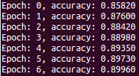
print("Epoch: %d, accuracy: %.5f" % (epoch, acc))
Load it up and run it! You should get results similar to this:
.
.
.
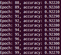
Wait a second, 92% is worse than the last article!
Yes it is. Why is that?
You have the tools you need to become an expert…time to earn some experience! Logistic regression models are great for making principled probabilistic predictions from arbitrary input features. But ultimately, logistic regression is just a linear model. Linear models are surprisingly useful, but if optical character recognition were solvable with a linear model, this problem would not have been worthy of study for the past two decades!
Science is iterative, and you just did an iteration! Congrats! Time to do another…what is your next hypothesis?
Visualization informs better models
To develop better models, you need to understand the strengths and deficiencies of your current model. We showed a simple version of this above, using grayscale distributions and visual inspection of a few examples. This is a good basic method, because every dataset has examples and distributions to inspect.
But optical character recognition is a visual task, and our human eyes + brains are very good at seeing visual patterns…can we exploit visualization to discover patterns of errors for this specific task? You be the judge! There are many examples MNIST visualizations. Here are a couple of our favorites, a creative take on the standard “confusion matrix” from @genekogan and @AlecRad:
Each element is the sample with the highest probability.
Model is a simple 1-layer neural network, trained on ~3k samples.
Accuracy is around 88%.
Image credit: Gene Kogan.
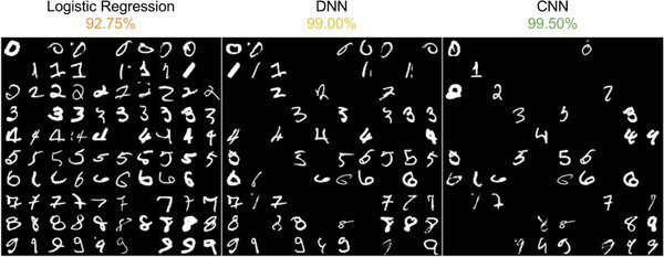
Comparing three different types of model:
(left) logistic regression, (mid) a multi-layered/deep neural network, (right) a convolutional neural network
Image credit: Alec Radford.
Next, we’ll show how to implement neural networks in Tensorflow. By changing a few lines of code to implement a more powerful model, we’ll go from about 92% accuracy to better than 99%.