Data visualization
A big part of working with data is getting intuition on what those data show. Staring at raw data points, especially when there are many of them, is almost never the correct way to tackle a problem. Low dimensional data are easy to visually inspect. You can simply pick pairs of dimensions and plot them against each other. Say, for example, I wanted to see how distance to a subway stop is correlated to house price — I’d make a plot. If the points were seemingly random, then there is no correlation. If the points follow some pattern (such as a line) then there is a correlation. However, as the number of dimensions increases, this technique makes less sense because 3D plots are a lot harder to read than 2D plots. Trying to compare four dimensions of data against each other is nearly impossible. So, what can we do?
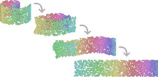
One strategy is to embed the high dimensional data into a smaller dimensional space. For visualization purposes, we generally try to reduce the number of dimensions to two. To build intuition, consider the following toy problem that has three dimensions. The input is points arranged in a curl. As humans, we can see that there is structure in this 3D representation, and we can use that structure to effectively unroll the 3D space and flatten it to a 2D space.
This is exactly what we want to do, except instead of using human intuition, we will use the power of machine learning. This style of operation is commonly called nonlinear dimensionality reduction, or manifold leaning. For more information I would recommend reading the Nonlinear Dimensionality Reduction Wikipedia page. In this article, I’m going to focus on one my favorite kinds of embedding algorithms: t-SNE.
t-Distributed Stochastic Neighbor Embedding (t-SNE) is one way to tackle these high dimensional visualization problems. Instead of trying to preserve the global structure like many dimensionality reduction techniques, t-SNE tries to group local data points closer to each other, which (in my experience) is a better match for building human reasoning. Part of the power of this technique is that it can normally be treated as a black box, and I’ll do just that for the remainder of this blog post. For those interested, I would highly recommend this fantastic Google Tech Talk which goes into a lot more detail.
Easy to use
In most cases, t-SNE just works. It’s implemented in many different computer languages — you can check which ones on Laurens van der Matten’s site. For Python users, there is a PyPI package called tsne. You can install it easily with pip install tsne.
To make use of this, we first need a dataset of some kind to try to visualize. For simplicity, let’s use MNIST, a dataset of handwritten digits. The code below uses skdata to load up mnist, converts the data to a suitable format and size, runs bh_tsne, and then plots the results.
import numpy as np
from skdata.mnist.views import OfficialImageClassification
from matplotlib import pyplot as plt
from tsne import bh_sne
# load up data
data = OfficialImageClassification(x_dtype="float32")
x_data = data.all_images
y_data = data.all_labels
# convert image data to float64 matrix. float64 is need for bh_sne
x_data = np.asarray(x_data).astype('float64')
x_data = x_data.reshape((x_data.shape[0], -1))
# For speed of computation, only run on a subset
n = 20000
x_data = x_data[:n]
y_data = y_data[:n]
# perform t-SNE embedding
vis_data = bh_sne(x_data)
# plot the result
vis_x = vis_data[:, 0]
vis_y = vis_data[:, 1]
plt.scatter(vis_x, vis_y, c=y_data, cmap=plt.cm.get_cmap("jet", 10))
plt.colorbar(ticks=range(10))
plt.clim(-0.5, 9.5)
plt.show()
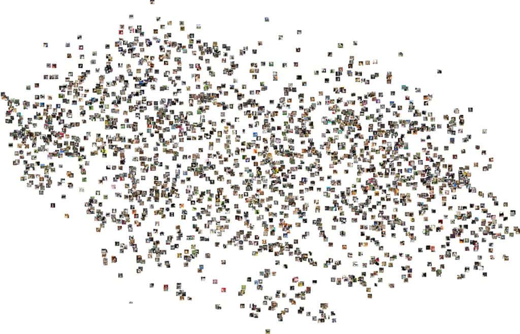
After about two minutes of execution, the result looks something like this: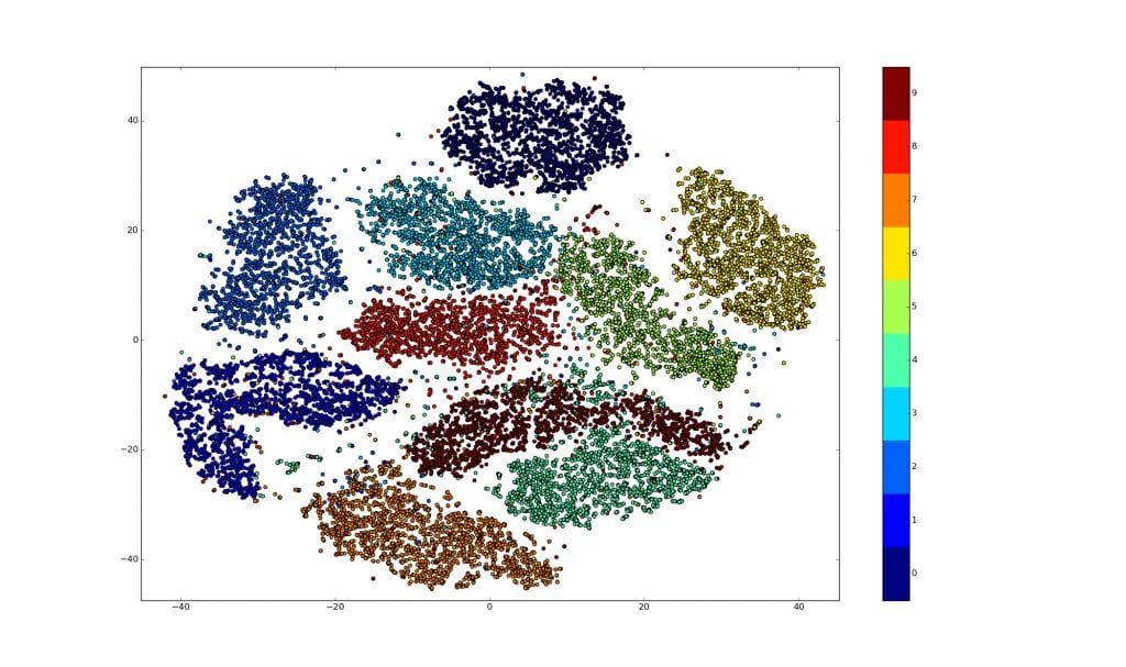 While MNIST is a really great dataset for testing and evaluating ideas, this a rather easy task. Let’s try t-SNE on something a little bit harder! Recently, Kaggle hosted an image processing competition titled Dogs vs. Cats.
Since these images are much more detailed, I would recommend clicking the images to download a higher resolution version for further exploration.
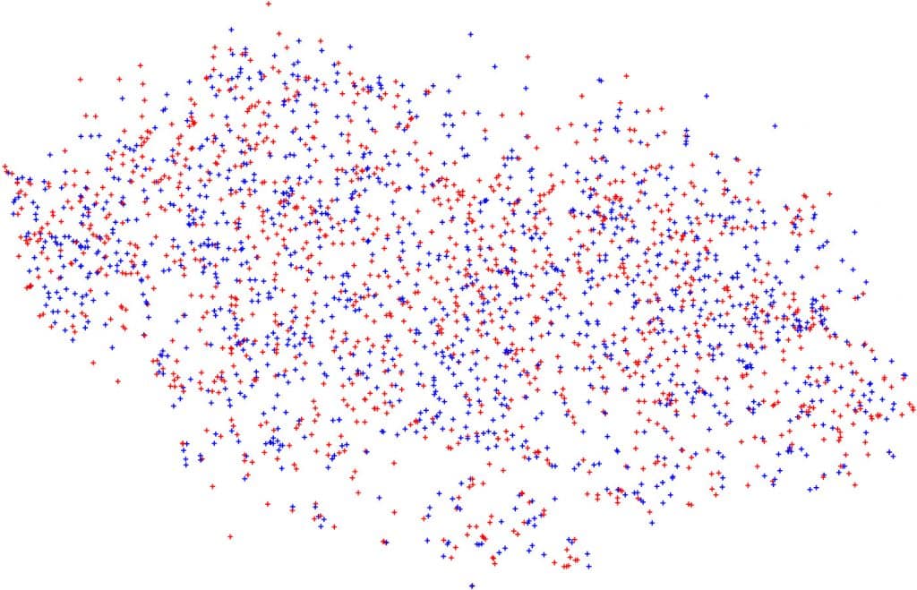
Now, these embeddings don’t look nearly as good, because they’re working on raw pixels values. In general, when we look at images, we look to patterns and objects, not pixel intensities at pixels. It’s asking too much of our dimensionality reduction algorithm to get all of that from just pixel values. So, how can we resolve this? Converting images into some representation that preserves the content of the image is a hard problem. These features strive to be invariant (they do not change) under certain constraints. For example, is a cat still a cat depending on the quality of a photo? Does the location of the cat in the image matter? A zoomed in version of a cat is still a cat. The raw pixel values may change drastically, but the subject stays the same.
There are a number of techniques used to make sense of images, such as SIFT or HOG, but computer vision research has been moving more towards using convolutional neural networks to create these features. The general idea is to train a very large and very deep neural network on an image classification task to differentiate between many different classes of images. In the processes of learning to classify, the model learns useful feature extractors that can then be used for other tasks. Sadly, these techniques require large amounts of data, computation, and infrastructure to use. Models can take weeks to train and need expensive graphics cards and millions of labeled images. Although it’s highly rewarding when you get them to work, sometimes creating these models is just too time intensive.
indico provides a feature extractor with its Image Features API, which is built using the same technique I desribed above: a stack of convolution layers trained on a 1000-way image classification task. To see the effect, we can apply the Image Features API to this dataset and then t-SNE the result to see how it performs against raw pixels.
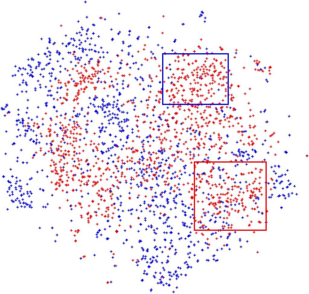
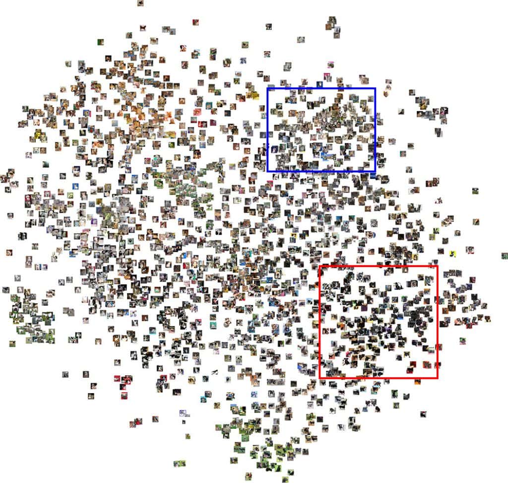
Right off the bat we can see that there is much more clustering based off of what is in the image. The features don’t just tell us which images are cats and which images are dogs, but instead group them and provide more information. Take the red and blue clusters. Both contain cats, but blue contains grey cats with stripes, while red contains black cats.
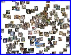
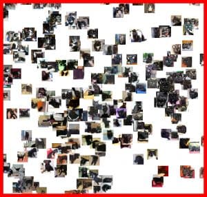
By working in a space that is better attuned for images, we can really start exploring and picking out interesting things in data!
Conclusion
The applications of t-SNE are limitless. It can be applied anytime there is a high dimensional dataset — it has been applied to text and natural language processing, speech, and even to visualize Atari game states.
Recently there has been a lot of hype around the term “deep learning“. In most applications, these “deep” models can be boiled down to the composition of simple functions that embed from one high dimensional space to another. At first glance, these spaces might seem to large to think about or visualize, but techniques such as t-SNE allow us to start to understand what’s going on inside the black box. Now, instead of treating these models as black boxes, we can start to visualize and understand them.
At Indico, we’ve begun adapting some of these techniques to commercial uses, where businesses and other organizations can access AI explainability for their process automation tasks. The Indico Platform structures this data, enabling you to build innovative, mission-critical enterprise workflows that maximize opportunity, reduce risk, and accelerate revenue.
Effective January 1, 2020, Indico will be deprecating all public APIs and sunsetting our Pay as You Go Plan.
Why are we deprecating these APIs?
Over the past two years our new product offering Indico IPA has gained a lot of traction. We’ve successfully allowed some of the world’s largest enterprises to automate their unstructured workflows with our award-winning technology. As we continue to build and support Indico IPA we’ve reached the conclusion that in order to provide the quality of service and product we strive for the platform requires our utmost attention. As such, we will be focusing on the Indico IPA product offering.
